GUI Overview

The normal graphical user interface (GUI) is organized around three main tasks: loading scans, inspecting detector images, and connecting image features to reciprocal-space coordinates for orientation and integration.

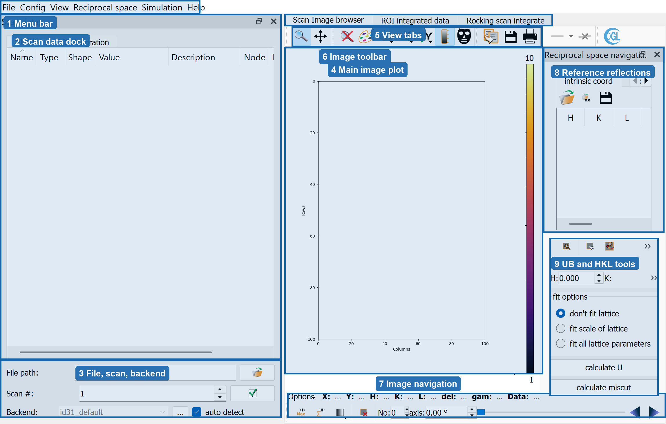
The screenshot below shows the default layout after starting orGUI with examples/config_minimal. The numbered regions are the main visible working areas.

1. Menu Bar

The menu bar provides access to application-level actions:

File

Open, refresh, and close Nexus/SPEC/log files; generate a scan from image files; load interlaced or segmented scans; and reload image data.

Config

Load machine and crystal configuration, open machine/crystal parameter dialogs, adjust CPU count and database compression, control automatic scan loading, select background images, and edit excluded images.

View

Toggle reference reflections, allowed Bragg reflections, ROI display, CTR reflections, and machine-parameter markers on the image plot.

Reciprocal space

Calculate available CTRs and open the orientation-matrix editor.

Simulation

Create a dummy scan for testing or demonstration.

Help

Open geometry and application information dialogs.

2. Scan Data Dock

The Scan data dock is the main scan-selection panel. Its NEXUS tab shows the loaded file tree through a Nexus/HDF5 browser. Double clicking a compatible scan node opens that scan.

The same dock also contains the ROI integration tab. That tab is not shown in the screenshot, but it is where ROI size, background ROI size, integration mode, correction options, and the ROI integrate scan action are configured. The available integration modes are:

• hklscan: stationary integration along H(s) = H_1 * s + H_0 in r.l.u.

• fixed: integration at a fixed detector-pixel ROI.

• rocking hklscan: rocking-scan integration along an HKL line.

• rocking Bragg: rocking-scan integration at calculated Bragg reflections.

3. File, Scan, And Backend Controls

These controls select the data source and loader:

File path

Path to a Nexus, SPEC, or log file.

Scan #

Scan number to load from the selected file. The button beside it opens the scan.

Backend

Beamline/file-format loader used to interpret the selected scan. With auto detect enabled, orGUI tries to infer the backend from the selected Nexus metadata. The ... button loads a custom backend file. See Beamline Backends for backend selection and custom backend files.

4. Main Image Plot

The Scan Image browser tab contains the central detector image plot. This area displays the current detector frame and overlays such as reference reflection markers, calculated Bragg/CTR reflections, machine-parameter markers, masks, and ROIs.

The plot coordinates are detector pixels. When a scan and calibration are available, orGUI also uses the image position and scan axis value to connect pixels to reciprocal-space coordinates.

5. View Tabs

The central workspace has three tabs:

Scan Image browser

Inspect raw detector images and overlays.

ROI integrated data

Plot integrated intensity curves and inspect integrated output data.

Rocking scan integrate

Work with the rocking-peak integration helper.

6. Image Toolbar

The toolbar above the image plot contains common plot and image tools from the plot widget, including zoom/pan-style navigation, colormap and display controls, mask tools, and save/print-style actions. These tools operate on the image plot currently shown in the Scan Image browser tab.

7. Image Navigation

The lower image toolbar controls the active frame and scan overlays:

Max / sum

Toggle display of the maximum image or summed image over the scan.

Transparency

Adjust the alpha value of the max/sum overlay.

Exclude image

Exclude the current image from max/sum image calculations.

No

Current image number.

axis

Current scan-axis value in degrees.

Slider and previous/next buttons

Move through images in the loaded scan.

8. Reference Reflections

The Reciprocal space navigation dock stores reference reflections used for orientation-matrix calculation and navigation. The visible intrinsic coord table stores H, K, L, detector x/y position, and image number. The neighboring SIXC angles tab shows calculated diffractometer angles for the selected reflections.

Useful actions in this area include:

• jump to the image associated with a selected reflection

• set the current image for a selected reflection

• perform a 2D peak search around a reflection

• add a suggested Bragg reflection when calculated candidates are available

Double clicking in the image plot can add or move reflection markers, depending on the active interaction mode.

9. UB And HKL Tools

The lower part of the Reciprocal space navigation dock contains the orientation and HKL tools. The visible HKL spin boxes and search action calculate where a requested reflection should appear. The fit options control how much the lattice is adjusted when calculating the orientation matrix:

don't fit lattice

Keep lattice parameters fixed and fit orientation from the selected reflections.

fit scale of lattice

Fit a lattice scale factor when enough reflections are available.

fit all lattice parameters

Fit all lattice parameters when enough reflections are available.

calculate U

Calculate the orientation matrix from the current reference reflections.

calculate miscut

Estimate the miscut from the deviation between the current orientation matrix and the ideal orientation.

Typical First Workflow

1. Load a configuration from Config -> Load config or start orGUI with a config file.

2. Select the scan file, scan number, and backend in the Scan data dock.

3. Open a scan and inspect the detector image in Scan Image browser.

4. Add or edit reference reflections in Reciprocal space navigation.

5. Click calculate U and verify that calculated reflections match observed image features.

6. Switch to ROI integration in the Scan data dock, set ROI parameters, and integrate the desired scan.